
Simulate
Ready-made physics and chemistry models, models you write as rate equations or formulas, fitting to data and simulation in the BO loop.
Running a model
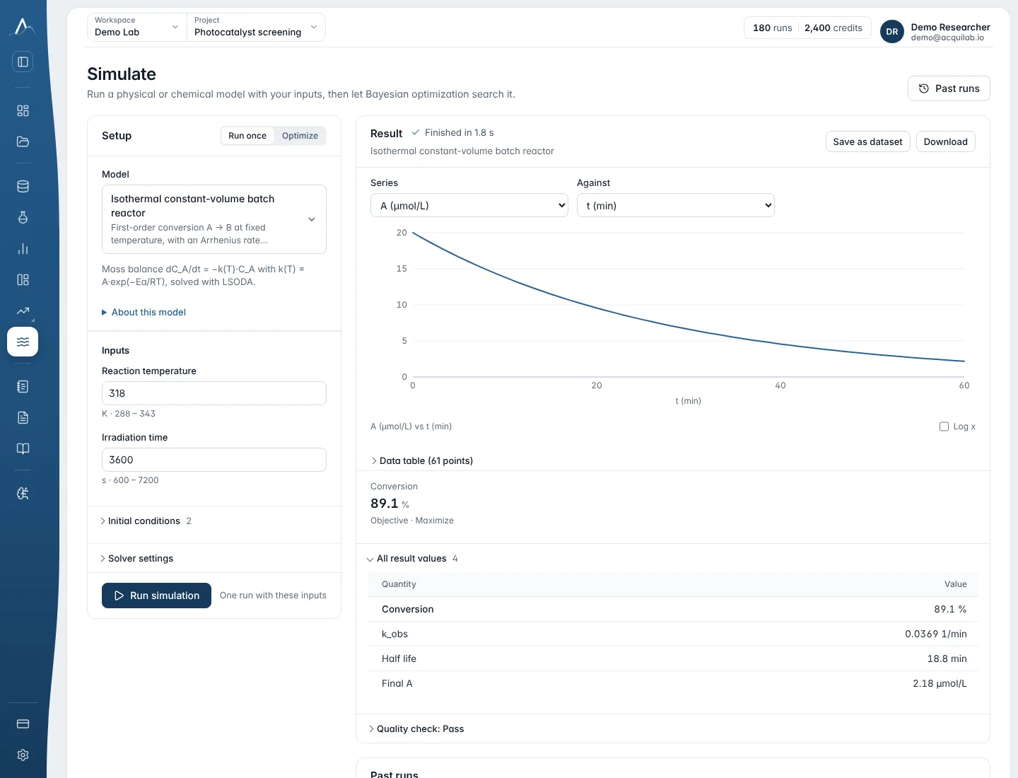
Simulate runs validated physics and chemistry models in an isolated worker with bounded time and memory, and records the model version and inputs with every result.
- In Setup, choose the model and change its inputs; units and allowed ranges are shown next to each. The model's description lists its assumptions, validity, known failure modes and citations.
- What to do: Run once, or Optimize to let Bayesian optimization run the model repeatedly (see Simulation in the BO loop).
- The result shows the values, curves and a quality check, with Download (CSV or JSON), Save as dataset and Open in Plot Studio.
- Past runs groups runs that belong together (compared sets, optimization loops, consecutive runs of one model). Reopen a run, compare 2–8 runs, or compare 2–10 runs with measured data on one graph.
Packages and limits
| Package | Models | What you can compute | Example inputs | Time limit |
|---|---|---|---|---|
| SciPy / NumPy (AcquiLAB model engine) | custom_ode, custom_algebraic, batch, CSTR, PFR, diffusion, heat, reaction–diffusion, membrane, electrode diffusion, Cottrell, Butler–Volmer, CV, EIS, isotherm, breakthrough | Rate equations over time (LSODA, switches between stiff and non-stiff methods), algebraic formulas, 1-D transport, reactor balances, electrode kinetics, impedance, adsorption | An enzyme cascade to maximum H₂O₂; CV at 10–1000 mV/s; a Nyquist plot for k⁰ = 0.01 cm/s | seconds to about 1.5 min |
| PySCF 2.14 (density functional theory) | dft_molecule | Kohn–Sham DFT with the PBEh(a) hybrid (Exc = a·ExHF + (1 − a)·ExPBE + EcPBE), a single point on the GFN2-xTB structure, SCF to 10⁻⁹ Eh: HOMO and LUMO energies, the HOMO–LUMO gap (objective), orbital energies, total energy; implicit solvent (ddCOSMO), ions and radicals | SMILES up to 40 atoms; basis def2-SVP (default), 6-31G*, STO-3G or def2-TZVP; exact exchange a = 0 (PBE) … 0.25 (PBE0, default) … 1; charge; unpaired electrons; solvent none, water, methanol, acetonitrile, DMSO or toluene | up to 30 min |
| tblite 0.7 (GFN-xTB) and RDKit 2026.3 | xtb_molecule | SMILES → 3D (RDKit ETKDG) → GFN2- or GFN1-xTB relaxed geometry, orbital energies, dipole, harmonic frequencies, the IR spectrum with intensities, thermochemistry G, H and S at T (RRHO, 1 atm) | SMILES up to 100 atoms of H, B, C, N, O, F, Si, P, S, Cl, Br, I; GFN2 or GFN1; ALPB solvent none, water, methanol, acetonitrile, DMSO, acetone, THF, toluene, hexane, CH₂Cl₂, CHCl₃; T 100–1500 K; symmetry number; IR band width | up to 30 min |
| OpenMM 8.6 | water_md | NPT molecular dynamics of a water box with PME: density, potential energy per molecule, ΔHvap, the O–O radial distribution g(r), self-diffusion coefficient | T 250–400 K; pressure; molecules; equilibration and production (ps); water model TIP3P, SPC/E, TIP4P-Ew, TIP3P-FB or TIP4P-FB | up to 30 min |
| Cantera 3.2 | combustion_equilibrium, ignition_delay | Adiabatic flame temperature and equilibrium products (Gibbs minimisation at constant H and P) with an equivalence-ratio sweep; ignition delay in a constant-pressure reactor with detailed chemistry | φ 0.3–3; T₀; pressure 0.5–60 atm; mechanism and fuel (validated for methane–air and H₂–air) | up to 2 min |
Quantum chemistry and molecular dynamics run on a separate chemistry worker with 4 GB of memory. A DFT or water MD run uses 5 runs, an xTB run 2, every other model 1 (see Runs).
Worked chemistry examples
| Question | Model and settings | What to read |
|---|---|---|
| HOMO–LUMO gap of phenol in water | dft_molecule · SMILES Oc1ccccc1 · def2-SVP · solvent water · a = 0.25 (PBE0) | HOMO, LUMO and gap (eV); compare with a gas-phase run to see the solvent shift |
| The gap shrinks with conjugation | dft_molecule · benzene c1ccccc1, naphthalene c1ccc2ccccc2c1, anthracene c1ccc2cc3ccccc3cc2c1 · same basis and a | Gap trend across the series (compare runs) |
| How much does the functional matter? | dft_molecule · one molecule · a = 0, 0.25, 0.5 | The gap grows with exact exchange; a = 0 is PBE, 0.25 is PBE0 |
| Push–pull dye, donor and acceptor levels | dft_molecule · 4-nitroaniline Nc1ccc(cc1)[N+](=O)[O-] · def2-SVP · water | HOMO (donor side) and LUMO (acceptor side) energies |
| A stable radical | dft_molecule or xtb_molecule · TEMPO CC1(C)CCCC(C)(C)N1[O] · unpaired electrons 1 | Orbital energies of the open-shell molecule |
| Which tautomer is favoured in water? | xtb_molecule · 2-hydroxypyridine Oc1ccccn1 against 2-pyridone O=c1cccc[nH]1 · GFN2 · water, then none | ΔG between the two (kJ/mol), and whether the solvent changes the order |
| A large dye cation | xtb_molecule · rhodamine B (64 atoms) · charge 1 · GFN2 | Relaxed structure, orbitals and the IR spectrum; a few minutes, well inside the 30-minute limit |
| Predict an IR spectrum | xtb_molecule · ethanol CCO (default) or CO₂ O=C=O | IR spectrum; CO₂ shows the IR-silent symmetric stretch |
| Water's density maximum | water_md · TIP4P-Ew · T 260–320 K | Density against T; g(r) peak near 0.28 nm; D ≈ 5·10⁻⁹ m²/s for TIP3P at 298 K |
| Hottest flame | combustion_equilibrium · methane–air · φ sweep 0.6–1.6 | Tad peaks slightly rich of φ = 1 (about 2226 K at φ = 1 for methane–air) |
| Ignition delay map | ignition_delay · T₀ 900–1400 K · P 1, 10, 40 atm · φ 1 | Arrhenius-like fall of the delay with T₀, shorter at higher P |
Ready-made models
23 models. The design inputs are what Bayesian optimization searches when you choose Optimize; the objective is fixed by the model.
| Model | Physics | Design inputs | Outputs | Objective | Example question |
|---|---|---|---|---|---|
| Reactors | |||||
batch_isothermal | dC/dt = ν·r(C), mass-action network at fixed T (Arrhenius rate constants) | temperature 200–600 K, final time | concentration profile, conversion, yield, selectivity | max yield | Best T and time for the intermediate in A → B → C |
cstr_steady | 0 = (Cin − C)/τ + ν·r(C) | temperature, τ | steady concentrations, conversion, yield, selectivity | max conversion | Residence time for 90 % conversion |
pfr_ideal | dC/dτ = ν·r(C), constant density | temperature, τ | exit concentrations, conversion, yield, selectivity | max conversion | PFR against CSTR for the same network |
| Electrochemistry | |||||
cottrell | I = nFAC√(D/πt) | area, D, C_bulk | I(t), j(t) | max current | Expected step current for a 3 mm disk |
butler_volmer | i = i₀[exp(αanFη/RT) − exp(−αcnFη/RT)] | i₀, η, temperature, area | j, I, Tafel branches | max current | Overpotential needed for 10 mA/cm² |
electrode_diffusion_1d | Planar diffusion to an electrode with a bulk boundary | area, D, C_bulk | C(x,t), I(t), flux | max current | When does Cottrell break down in a thin cell? |
cyclic_voltammetry | Diffusion of O and R with Butler–Volmer flux, linear sweep | scan rate 0.001–10 V/s, k⁰, C_bulk | I against E, ipc, ΔEp, ipa/ipc | max cathodic peak | ΔEp against scan rate to judge reversibility |
eis_randles | Rs + (Cdl ∥ (Rct + Warburg)) | R_s, k⁰, C_dl | Nyquist, Bode, |Z|, phase, Rct | min low-frequency impedance | Semicircle size for a faster electrode |
| Transport and heat | |||||
diffusion_1d_steady | 0 = D d²C/dx² | D | C(x), boundary fluxes | max flux | Steady flux through a gel layer |
diffusion_1d_transient | ∂C/∂t = D ∂²C/∂x² | D | C(x,t), fluxes | max flux | Time to reach a sensor surface |
reaction_diffusion_1d | ∂Cᵢ/∂t = ∇·(Dᵢ∇Cᵢ) + ωᵢ(C) | D, k | C(x,t), boundary flux | max uptake flux | Enzyme layer thickness against substrate penetration |
membrane_1d | Fickian slab with partition K at both faces | D, C_upstream, C_downstream | C(x), flux, permeability | max flux | Permeability of a coating |
heat_conduction_1d_steady | d/dx(k dT/dx) = 0 | k | T(x), heat flux | max heat flux | Insulation thickness |
heat_conduction_1d_transient | ρcp∂T/∂t = ∂/∂x(k ∂T/∂x) | k (plus ρ, cp, target T) | T(x,t), centre T, time to temperature | max centre T | Time for a sample to reach 60 °C |
| Separations | |||||
adsorption_isotherm | Sips (Langmuir–Freundlich) with van 't Hoff temperature dependence; n = 1 is Langmuir | temperature 200–600 K, C_feed | q(C), θ, q at feed | max loading | Loading at 25 against 60 °C |
fixed_bed_breakthrough | Axially dispersed plug flow, LDF uptake and a Sips isotherm | u 1e-5–0.5 m/s, L 0.01–10 m | Cout(t), C/C₀, breakthrough time, productivity | max productivity | Column length and velocity for the best productivity |
| Combustion and molecules | |||||
combustion_equilibrium | HP equilibrium (Cantera) | φ 0.3–3, T₀ 250–1200 K | Tad(φ), products | max flame T | Flame temperature against mixture |
ignition_delay | Constant-pressure adiabatic reactor (Cantera, CVODES) | T₀ 800–2000 K, P 0.5–60 atm, φ | T(t), delay | min delay | Delay at engine-like conditions |
xtb_molecule | GFN-xTB (tblite) on an RDKit structure | temperature 100–1500 K | IR spectrum, G, orbitals, dipole | min G | Tautomer or conformer energy |
dft_molecule | Kohn–Sham DFT, PBEh(a) (PySCF) | exact exchange 0–1 | orbital energies, gap | max gap | HOMO–LUMO gap of a dye |
water_md | NPT molecular dynamics with PME (OpenMM) | temperature 250–400 K | gOO(r), density | max density | Temperature of maximum density |
| Models you write | |||||
custom_ode | dy/dt = f(y, t, p), whitelisted expressions, SciPy LSODA | your parameters (1–6 at a time) | every state's curve and one reported value | max or min of the report | See the ODE library below |
custom_algebraic | Outputs as formulas of the parameters | your parameters | outputs and one reported value | max or min of the report | See the formula library below |
Fit to measured data
Fitting works for batch reaction kinetics, EIS Randles, the adsorption isotherm, fixed-bed breakthrough and custom_ode: choose 1–6 parameters with bounds and a measured column in the project (in the same units as the model), optionally a σ column. The fit uses 10–400 model evaluations and counts as one simulation. It reports the values with intervals, and the fitted curve can be saved as a dataset.
Writing your own model
When no ready-made model fits (an enzyme cascade, a reaction network, a dose–response), write the rate equations yourself as custom_ode, or plain formulas as custom_algebraic. AcquiLAB evaluates them with a whitelist of operations, never arbitrary code, and integrates them with SciPy's LSODA solver.
The system, part by part
- states: 1–8 quantities that change, each
{name, initial, unit}. - rates: one
d(state)/dtexpression per state. - parameters: up to 24 constants
{name, value, unit, source}; the source is the paper, or"assumed". - report: the headline number, an expression evaluated at the end of the run. Optimization maximises or minimises it.
- time:
{end, unit: s | min | h, points}. Every state's curve is kept.
Rules the checker enforces
- Allowed: numbers, names,
+ - * /,**with a plain positive number up to 8,sin cos exp log log10 sqrt abs min max tanh sinh cosh,pi,e. - Rates are per second, and
tis in seconds, whatever unit you choose for the run time. - Reserved names:
y,t,k(ODE),x(formulas), function names,pi,e. Usek1,kf,kcat… - Exponents must be plain numbers:
S**nHis refused. Writeexp(nH*(log(K) - log(max(S, 1e-12))))instead. - Guard
logorsqrtof a changing quantity:log(max(A, 1e-12)),sqrt(max(A, 0)). - No if/else, comparisons or events. For a switch use a smooth step:
0.5*(1 + tanh((t0 - t)/w)). - Units are not converted. Keep them consistent yourself (mM with mM/s, and so on).
Full example: the creatinine sensing cascade (CA → CI → SOX)
The model behind the 4 October 2026 run in the Creatinine sensor project, with the literature constants used there. It passed AcquiLAB's checker together with the optimization settings below (total enzyme fixed at 3 µM, 20 runs). That run found an optimum near 1 : 1.3 : 1.7 (CA : CI : SOX), 0.0196 mM H₂O₂ at 5 min against 0.0186 mM for 1 : 1 : 1, with sarcosine oxidase as the rate-limiting step.
{
  "states": [
    {"name":"Cn",  "initial":0.1,  "unit":"mM"},   // creatinine
    {"name":"Cr",  "initial":0,    "unit":"mM"},   // creatine
    {"name":"Sar", "initial":0,    "unit":"mM"},   // sarcosine
    {"name":"O2",  "initial":0.25, "unit":"mM"},
    {"name":"H2O2","initial":0,    "unit":"mM"}],
  "parameters": [
    {"name":"kcat1","value":252, "unit":"1/s","source":"BRENDA, P. putida creatininase"},
    {"name":"Km1",  "value":26,  "unit":"mM", "source":"J Biochem 1979"},
    {"name":"Kcr",  "value":130, "unit":"mM", "source":"J Biochem 1979"},
    {"name":"Keq",  "value":1.3, "unit":"1",  "source":"assumed"},
    {"name":"kcat2","value":10.5,"unit":"1/s","source":"derived from 14 U/mg"},
    {"name":"Km2",  "value":1.33,"unit":"mM", "source":"BRENDA"},
    {"name":"kcat3","value":14,  "unit":"1/s","source":"J Appl Biol Sci 33:161"},
    {"name":"Km3",  "value":3.6, "unit":"mM", "source":"J Appl Biol Sci 33:161"},
    {"name":"KmO2", "value":0.1, "unit":"mM", "source":"assumed"},
    {"name":"E1","value":0.001,"unit":"mM","source":"assumed"},
    {"name":"E2","value":0.001,"unit":"mM","source":"assumed"},
    {"name":"E3","value":0.001,"unit":"mM","source":"assumed"}],
  "rates": {
    "Cn":  "-kcat1*E1*(Cn - Cr/Keq)/Km1/(1 + Cn/Km1 + Cr/Kcr)",
    "Cr":  "kcat1*E1*(Cn - Cr/Keq)/Km1/(1 + Cn/Km1 + Cr/Kcr) - kcat2*E2*Cr/(Km2 + Cr)",
    "Sar": "kcat2*E2*Cr/(Km2 + Cr) - kcat3*E3*Sar/(Km3 + Sar)*O2/(KmO2 + O2)",
    "O2":  "-kcat3*E3*Sar/(Km3 + Sar)*O2/(KmO2 + O2)",
    "H2O2":"kcat3*E3*Sar/(Km3 + Sar)*O2/(KmO2 + O2)"},
  "report": {"name":"H2O2 at 5 min","expression":"H2O2","unit":"mM"},
  "time":   {"end":5,"unit":"min","points":301}
}

// optimize the enzyme split at a fixed total of 3 µM
optimize    = [{"name":"E1","lower":0.0002,"upper":0.0026},
               {"name":"E2","lower":0.0002,"upper":0.0026},
               {"name":"E3","lower":0.0002,"upper":0.0026}]
constraints = [{"sum":["E1","E2","E3"],"equals":0.003}]
goal = "maximize", max_simulations = 20
Comments (//) are for reading only; leave them out of the real JSON.
Run once
Simulate → custom ODE, or run_written_simulation. Gives every state's curve and the reported value.
Compare 2–6 variants
The same system with some values changed, started together: variants=[{"label":"1:2:1","values":{"E2":0.0015}}].
Optimize 1–6 parameters
Ranges, up to 4 constraints (sum … equals / at_most / at_least, or coefficients with eq, le or ge), 6–40 simulations.
Fit to measured data
1–6 parameters with bounds, a measured column in the project, in the same units as the system.
Custom ODE library
Every row was written in AcquiLAB's format and passed its checker. Copy a rate, give the parameters values and sources, and you have a runnable model. Up to 8 states fit in one system, so rows can be combined (for example a cascade plus enzyme inactivation).
| System | States | Rate expressions (AcquiLAB syntax) | Typical report | Question to ask, or optimization target |
|---|---|---|---|---|
| Enzymes and biosensors | ||||
| Michaelis–Menten | S, P | S: -kcat*E*S/(Km + S)P: kcat*E*S/(Km + S) | P at end | Enzyme amount for 90 % conversion in 10 min |
| Competitive inhibition | S, P | S: -kcat*E*S/(Km*(1 + I0/Ki) + S) | P at end | Compare 0, 50 and 200 µM inhibitor as variants |
| Mixed / uncompetitive inhibition | S | S: -Vmax*S/(Km*(1 + I0/Kic) + S*(1 + I0/Kiu)) | S left | Which inhibition type explains your progress curve (fit) |
| Substrate inhibition (Haldane) | S, P | S: -Vmax*S/(Km + S + S**2/Ksi) | P at end | Starting substrate that maximises product |
| Product inhibition | S, P | S: -Vmax*S/(Km*(1 + P/Kp) + S) | P at end | When product removal pays off |
| Cooperative (Hill) kinetics | S, P | S: -Vmax/(1 + exp(nH*(log(K05) - log(max(S, 1e-12))))) | P at end | Effect of nH on a switch-like response |
| Enzyme inactivation during use | E, S | E: -kd*ES: -kcat*E*S/(Km + S) | S left | Sensor drift; operational half-life ln2/kd |
| Two-substrate oxidase with HRP readout (GOx) | Glc, O2, H2O2, Res | Glc: -kcat*Eg*Glc*O2/(KmO*Glc + KmG*O2 + Glc*O2)H2O2: (same) - kHRP*H2O2Res: Iapp*kHRP*H2O2 | resorufin formed | Is O₂ limiting at high glucose? |
| Multi-enzyme cascade (creatinine CA–CI–SOX) | Cn, Cr, Sar, O2, H2O2 | reversible Haldane step + two MM steps + O₂ term (full JSON above) | H₂O₂ at readout | Best enzyme ratio at a fixed total (constraint sum = total) |
| Surface adsorption on an electrode (Langmuir kinetics) | th | th: kads*Cb*(1 - th) - kdes*th | coverage | Incubation time to 95 % coverage |
| Ligand–receptor binding (SPR-type) | L, Rf, LR | LR: kon*L*Rf - koff*LRL, Rf: -kon*L*Rf + koff*LR | LR/(LR + Rf) | KD = koff/kon; association time |
| Chemical kinetics | ||||
| Consecutive A → B → C with Arrhenius | A, B, C | A: -A1*exp(-Ea1/(R*T))*AB: A1*exp(-Ea1/(R*T))*A - A2*exp(-Ea2/(R*T))*B | yield of B | T and time that maximise the intermediate |
| Reversible A ⇌ B | A, B | A: -kf*A + kr*B | B at end | Approach to equilibrium, K = kf/kr |
| Second order A + B → P | A, B | A: -k2r*A*BB: -k2r*A*B | conversion | Effect of excess B |
| Autocatalysis A + B → 2B | A, B | A: -kau*A*BB: kau*A*B | B at end | Induction time against seed amount |
| Linear temperature ramp | A | A: -A1*exp(-Ea/(R*(T0 + ramp*t)))*A | A left | Ramp rate (K/s) for full conversion |
| Photodegradation with light absorption | C | C: -phi*Iabs*(1 - exp(-2.303*eps*lp*C)) | C left | Irradiation time; inner-filter effect |
| Free-radical polymerisation (QSSA) | In, Mo | In: -kdec*InMo: -kp*Mo*sqrt(2*fe*kdec/kt)*sqrt(max(In, 0)) | 1 − Mo/M0 | Initiator amount for 90 % conversion |
| Oscillating reaction (Brusselator) | X, Y | X: a - (b + 1)*X + X**2*YY: b*X - X**2*Y | X at end | Oscillations appear when b > 1 + a² |
| Bioprocess, ecology, epidemiology | ||||
| Monod fermentation | X, S, P | X: mumax*S/(Ks + S)*XS: -mumax*S/(Ks + S)*X/YxsP: Ypx*mumax*S/(Ks + S)*X | product titre | Feed substrate and inoculum for the highest titre |
| Logistic growth with Luedeking–Piret product | X, P | X: mu*X*(1 - X/Xmax)P: aLP*mu*X*(1 - X/Xmax) + bLP*X | titre | Growth- against non-growth-associated production |
| Predator–prey (Lotka–Volterra) | Prey, Pred | Prey: alpha*Prey - beta*Prey*PredPred: delta*Prey*Pred - gam*Pred | population | Phage–bacteria or grazing cycles |
| SIR / SEIR epidemic | S, E, I, R | S: -b0*S*IE: b0*S*I - sig*EI: sig*E - g0*IR: g0*I | I + R | Final size against R₀ = b0/g0 |
| Pharmacokinetics and release | ||||
| One compartment, oral dose | Agut, Cp | Agut: -ka*AgutCp: F*ka*Agut/Vd - ke*Cp | Cp at time | Dose giving a target trough at 12 h |
| Two compartments, IV bolus | C1, C2 | C1: -(k10 + k12)*C1 + k21*C2C2: k12*C1 - k21*C2 | C1 at time | Distribution against elimination phase |
| Infusion that stops (smooth switch) | Ci | Ci: Rin*0.5*(1 + tanh((tinf - t)/w)) - k10*Ci | C at end | Infusion length for a target level |
| Effect compartment (PK/PD) | Ce | Ce: ke0*(Ci - Ce) | Ce | Delay between plasma level and effect |
| Dissolution (Noyes–Whitney) | Md | Md: kdis*(Cs - Md/Vm) | dissolved mass | Time to 80 % release |
| Adsorption, energy and heat | ||||
| Pseudo-first-order adsorption | q | q: k1a*(qe - q) | q at end | Contact time for equilibrium |
| Pseudo-second-order adsorption | q | q: k2*(qe - q)**2 | q at end | Fit k2 and qe to uptake data |
| Battery, 1-RC Thevenin model | SOC, V1 | SOC: -I/QV1: I/C1 - V1/(R1*C1)report: E0 + Es*SOC - V1 - I*R0 | terminal voltage | Current that keeps V above cut-off for 1 h |
| Supercapacitor charging (RC) | Vc | Vc: (Vs - Vc)/(Rs*Cap)report: 0.5*Cap*Vc**2 | stored energy | Charge time to 95 % |
| Lumped heating (Joule and loss) | Tc | Tc: (Pj - hA*(Tc - Tamb))/mcp | T at end | Power for a 37 °C chip |
| Periodic forcing (day–night, AC) | Tf | Tf: (Tm + dT*sin(2*pi*t/Per) - Tf)/tau | T at end | Damping of a temperature swing |
Formula library
custom_algebraic has parameters, named outputs (up to 8) and a report, with no states or time. Use it for closed-form relations, or as a fast objective inside an optimization loop. Non-integer powers are written as exp(n*log(...)), and x is reserved. A system holds at most 24 parameters, so split large formula sets.
| Relation | Expression | Use |
|---|---|---|
| Randles–Ševčík peak current | 0.4463*n*F*A*Cb*sqrt(n*F*v*D/(R*T)) | Expected CV peak; compare with the measured ip |
| Hill dose–response | Emax/(1 + exp(nH*log(EC50/C))) | Response at a dose; dose for 80 % effect |
| Arrhenius | Apre*exp(-Ea/(R*T)) | Rate constant at a temperature |
| Eyring | kB*T/hP*exp(-dG/(R*T)) | Rate from an activation free energy (DFT or xTB ΔG‡) |
| Nernst | E0 + R*T/(n*F)*log(Cox/Cred) | Electrode potential |
| Beer–Lambert | eps*lp*Cm | Absorbance; concentration for A = 1 |
| Henderson–Hasselbalch | pKa + log10(Abase/HA) | Buffer pH |
| Langmuir isotherm | qm*bL*Ce/(1 + bL*Ce) | Loading |
| Freundlich isotherm | KF*exp(log(Ce)/nF) | Loading with a non-integer exponent |
| Q10 temperature scaling | r1*exp((T2 - T)/10*log(Q10)) | Biological rate at another temperature |
| Limit of detection | 3.3*sb/slope | LOD from the blank SD and the sensitivity |
| Stokes–Einstein | kB*T/(6*pi*eta*rh) | Diffusion coefficient of a particle |
Simulation in the BO loop
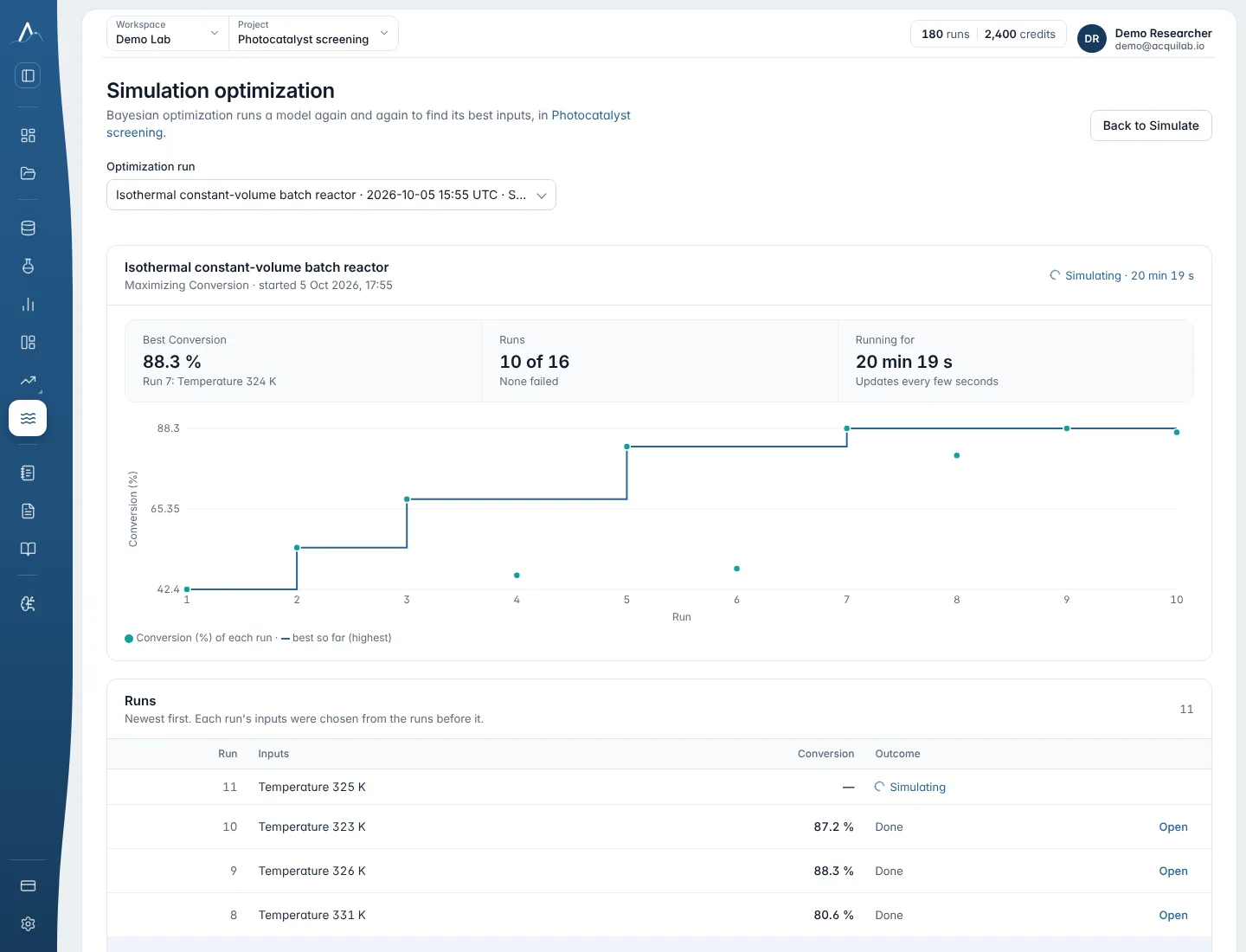
Choose a model, then What to do → Optimize. Bayesian optimization runs the model repeatedly, choosing each new set of inputs from the results so far. Settings stay as they are; only the inputs inside the search ranges change.
| Setting | Choices |
|---|---|
| Goal | The model's objective, for example maximise the HOMO–LUMO gap |
| Number of runs | 2–100 for a ready-made model; the first few are spread across the ranges and the model chooses the rest |
| Each run | Starts automatically, or waits for my approval |
| Model (more options) | Improved (recommended) or Simpler (standard 0.1.0) |
| Result scale | Choose from the results (default), as measured, or logarithm (results must be positive) |
| Spread-out starting runs | How many runs come before the model starts choosing |
| Exploration | Balanced, explore more (new regions), or refine the best result |
| Stop early | When a result reaches a target, or after a number of runs without improvement |
The loop page follows each run. Pause, resume, stop, or approve and skip single runs (a reason is optional). The loop reserves its whole run budget when it starts and gives back what it did not use.
Written-model loop
Optimize 1–6 parameters of your own system, with up to 4 linear constraints, in 6–40 simulations (Simulate, or start_written_model_optimization). Each iteration runs your system with the recommended values, and AcquiLAB checks that the stored run used exactly those values before it counts. To minimise, the loop maximises the negative.
Simulation as a guide to lab BO
Turn on Use simulation results as a guide in a lab campaign with the Improved model. Simulation results become a second, cheaper source; the model check reports how well simulation agrees with the lab, and only lab results can be the best.
Constraints are available for written models; a loop on a ready-made model searches its design inputs within the ranges you narrow.