
Analyze
From an instrument file to a result with units and uncertainties: techniques, methods, options and what to do when a run fails.
From file to figure
The normal path is four steps: Analyze → technique → upload → Analyze, and Plot Studio opens on the result.
The Analyze page shows one card per technique: General analysis, Spectroscopy, Electrochemistry, Materials, Imaging, and Separation & MS. Each card lists the methods it covers and what the analysis gives, and the search box matches methods, instruments and outputs (for example “qNMR”, “Scherrer” or “LOD”). Below the cards, Recent analyses lists the project's latest files with their state and headline result, with Open or Fix and re-run.
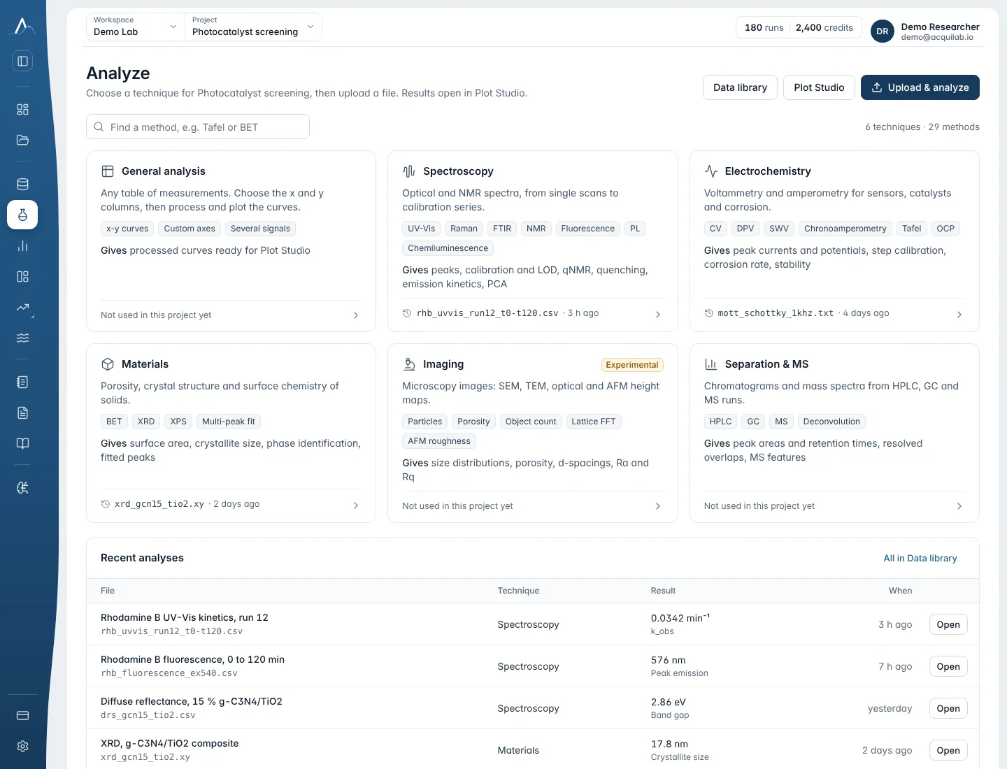
- Choose the technique card, then the method under it.
- Upload the file: CSV, TXT or XLS for tables, TIFF for images, JSON for the structured materials and MS exports. Instrument text exports with metadata lines (JASCO and similar) are read as they are; you don't need to edit the file. Several files at once work for Calibration from spectra and PCA: they are placed side by side, one column per file.
- Check the options. Columns are chosen from the header when the names are clear (for example
E (V),Ewe/V,<I>/mA,Abs); otherwise you pick them from the preview. Usea.u.for arbitrary units and1for dimensionless. - Press Analyze. Plot Studio opens with the result.
Methods
39 entries: 33 methods and the default analyzer of each technique. Every method reports values with units and, where the method defines them, uncertainties. Results are computed on the server; nothing in the browser recomputes them.
| Method | What it gives you | Input | Main options |
|---|---|---|---|
| General analysis | |||
| General x–y analysis | Processed curves of any table of measurements, ready for Plot Studio (for example the area under the curve). | CSV, TXT or XLS table | x and y columns with units (a.u. for arbitrary units, 1 for dimensionless) |
| Spectroscopy | |||
| Spectroscopy (technique default) | UV-Vis style spectrum processing and peak positions. | CSV, TXT or XLS | — |
| Analyze a curve on the graph | Pseudo-Voigt peak fit, area under the curve, Savitzky–Golay smoothing or 1st/2nd derivative, or a baseline offset, over a chosen X range. | X and Y columns, at least 5 points in the range | what to do, X range, window (5–101 points, odd), polynomial order, peak near X |
| Baseline correction | Subtracts a baseline that follows the lower edge of the curve (asymmetric least squares) or a flat offset; gives the corrected curve to plot or analyse further. | X column (wavelength, wavenumber, shift, time …) and Y column | baseline type, stiffness (flexible, medium, stiff), how strictly it stays under peaks, X range |
| Calibration curve (Beer–Lambert) | Straight-line fit of absorbance against concentration with residuals; slope ± SE, intercept, R², an unknown's concentration ± u. | Table of standards (at least 3 rows) | concentration and absorbance columns, unit, absorbance of an unknown |
| Calibration from spectra | Overlays the standards, reads each at the maximum, minimum, a wavelength or an area, fits the line and reads unknowns back. | Several files, or one wide table | signal kind, feature, range, concentrations (or units in column names), unknown columns |
| PCA of spectra | Scree plot, loadings against wavelength and the score plot. | Wide table, at least 3 spectra | axis in nm or cm⁻¹, 2–5 components, SNV, unit-length or maximum normalisation |
| Raman bands | Cosmic-ray removal, AsLS baseline and smoothing; band positions, heights and widths; pseudo-Voigt fits of the strongest bands. | Raman shift (cm⁻¹) and intensity | cosmic rays, baseline, smoothing, normalise, bands to fit (0–12), prominence |
| FTIR / IR bands | %T or T converted to absorbance, baseline, band positions and widths, fits. | Wavenumber and A or T | signal type, baseline, smoothing, bands to fit |
| Band assignment (suggested functional groups) | Suggests functional groups for bands above 1500 cm⁻¹ (O–H, N–H, C–H, C≡N, C=O …) from 27 group-frequency ranges. Screening, not identification. | FTIR spectrum | signal type, baseline, smoothing |
| Fluorescence / emission spectrum | Emission maximum, FWHM, centroid, integrated intensity, all peaks and an optional I(λ1)/I(λ2) ratio. | Wavelength and intensity | emission or excitation, wavelength range, baseline, normalise, ratio wavelengths |
| Fluorescence quenching (Stern–Volmer) | F₀/F = 1 + K_SV[Q]: K_SV ± u and R². | [Q] and intensity (at least 3 rows) | concentration unit, F₀ |
| Photoluminescence (PL) | Peak wavelength and photon energy, FWHM in nm and eV, integral, Stokes shift. | Wavelength and PL (absorption optional) | reference column and kind, baseline, smoothing |
| Chemiluminescence / emission kinetics | Maximum, time to maximum, total light, first-order decay fit and half-life. | Time and intensity | time unit, decay fit, background |
| NMR peaks and integrals | Peak list (shift, height, width in Hz) and integrals in protons relative to the first range. | ppm and intensity (MestReNova or TopSpin CSV) | nucleus ¹H, ¹³C, ¹⁹F or ³¹P, solvent, referencing, integral and leave-out ranges, MHz |
| qNMR purity (internal standard) | Purity in % w/w from the analyte and internal-standard integrals, proton counts, molar masses and weighed masses. | Quantitative ¹H spectrum | both ppm ranges, protons, molar masses, masses, standard purity |
| Reaction conversion by NMR | Conversion from reactant and product signals per proton. | ¹H spectrum of the mixture | both ranges and proton counts |
| Impurity and residual-solvent screening (¹H) | Flags residual solvents and common impurities for the chosen solvent and lists unexplained peaks. | ¹H spectrum | your compound's ranges, S/N threshold |
| Peak types and J couplings | s, d, t, q … m with J in Hz (first-order patterns). | 1D spectrum and spectrometer MHz | largest coupling, S/N, leave-out ranges |
| Electrochemistry | |||
| Electrochemistry (technique default) | Technique analyzer for potentiostat exports. | CSV, TXT or XLS | — |
| Cyclic voltammetry peaks | Per cycle: E_pa, i_pa, E_pc, i_pc, ΔE_p, E_mid and |i_pa/i_pc|. | E and I in recorded order | units, smallest peak (default 5 % of the range) |
| Chronoamperometry / chronopotentiometry | Charge after the step, Cottrell plot and D; or baseline, steady state, change and t50/t90/t95 for a step inside the trace. | Time and current or potential | where the step is, steady-state %, n, area, concentration |
| Differential pulse / square-wave voltammetry peaks | Checks the pulse sequence, linear background, peak potential, height, FWHM and area. | E and (difference) current | technique, pulse amplitude, width or frequency, step, polarity |
| Tafel analysis (corrosion) | E_corr, j_corr and the anodic and cathodic Tafel slopes. | Polarization curve | units, area, reference electrode, fit ranges (automatic 60–180 mV) |
| Calibration from injection steps (amperometric sensor) | Stable current (mean ± SD) before each injection, calibration line, sensitivity, R² and LOD. | One chronoamperometry recording with injections | concentration per step, window, injection times (automatic) |
| Materials | |||
| Materials (technique default) | Materials analyzer (for example XRD patterns) for the structured JSON export. | JSON | — |
| BET surface area | BET range by the Rouquerol criteria, S_BET ± u, C constant and monolayer capacity. | p/p₀ and amount adsorbed | unit, gas N₂, Ar or Kr, temperature, cross-section |
| XRD peaks, d-spacings and crystallite size | Finds and fits the diffraction peaks (pseudo-Voigt): 2θ, d-spacing, width and Scherrer crystallite size of each peak; Williamson–Hall size and strain from four or more peaks. | Powder pattern: 2θ (degrees) and intensity | X-ray tube (Cu, Co, Mo, Cr, Fe) or another wavelength, background, smallest peak, peaks to fit, Scherrer K, instrument broadening, 2θ range |
| XRD phase identification (against your references) | Ranks the reference patterns you supply by how well they match (whole-pattern similarity and peak positions). Candidate screening: a phase that is not among your references can't be found. | One table on the same 2θ points: 2θ, your pattern, one column per reference phase (for example simulated from CIF files) | X-ray tube or wavelength, peak position tolerance, weight of the whole-pattern similarity, smallest peak |
| Fit several peaks at once | Fits overlapping peaks together (pseudo-Voigt) after an optional straight or Shirley background: position, width, area and area % of each peak with standard errors, the fit and its residual. | X and Y columns covering the peaks (XPS, Raman, IR, UV-Vis, XRD, chromatography …) | peak positions (optional), number of peaks, smallest peak, background (straight, Shirley for XPS, none), X range |
| Imaging | |||
| Imaging · Microscopy (technique default) | Image summary and measurements from TIFF microscopy images. | TIFF | — |
| Particles in an image (count and size) | Separates particles from the background by a threshold (touching particles split): number, covered area fraction, median diameter and number per area. | Greyscale TIFF (SEM, optical …), bright particles on a darker background | pixel size and unit, threshold, smoothing, smallest particle, split touching particles, leave out particles cut by the edge |
| Porosity from an image | Takes the dark phase as pores: porosity (area fraction) and median pore size (local thickness). | Greyscale TIFF of a cross-section or membrane, darker pores | pixel size and unit, threshold, smoothing, smallest pore |
| Count objects in a fluorescence image | Counts bright objects (cells, nuclei, colonies, droplets …): number, number per area and how many touch the edge. | Greyscale TIFF, one channel, bright objects on a dark background | pixel size and unit, threshold, smoothing, smallest object, split touching objects, what the objects are |
| Lattice spacings from an HRTEM image (FFT) | Fourier transform of a lattice image: the spots, lattice d-spacings and the angle between two lattice directions. Screening, not crystallographic indexing. | Square-ish HRTEM or STEM TIFF with lattice fringes | pixel size and unit, window before the FFT (Hann or none), smallest spot, maximum number of spots |
| AFM roughness and topography | Areal roughness Sa and Sq, the height distribution (percentiles) and the number of raised features. | AFM height image as TIFF (heights as pixel values, for example exported from Gwyddion) | pixel size and unit, height unit, height that counts as a raised feature, smallest feature |
| Separation & MS | |||
| Separation & MS · Mass spectrum (technique default) | Centroid peaks with a noise baseline; mass spectrum profile with sticks. | JSON export | — |
| Chromatogram peaks and areas (integration) | Baseline, peak detection and integration: retention time, height, area and area %, width, tailing factor, plate count and resolution of each peak. | Time and detector signal (HPLC, GC, IC, SEC …) | baseline (straight, curved, none), regions kept out of the baseline, smoothing, smallest peak, integration width, minimum peak distance, peak direction, time range |
| Deconvolution of overlapping peaks | Separates co-eluting or shouldering peaks into Gaussian components on a straight local baseline: retention time, height, width, area and area % of each, with the fit and its quality. | Time and signal; a time window around the overlap | time window, retention times of the components (optional), number of components, shared or separate widths, how far a centre may move |
A technique card marked Experimental or Beta is still being checked against reference data. Every result records the method, its version and its scientific maturity.
Reading a result
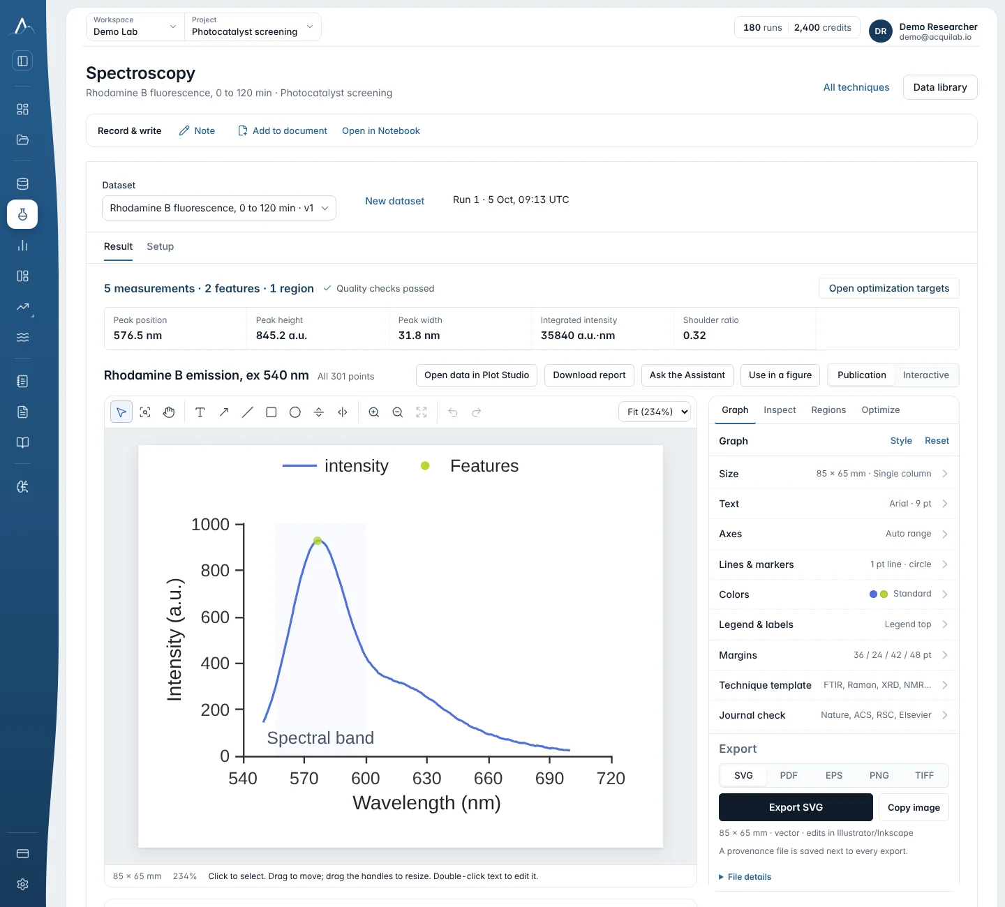
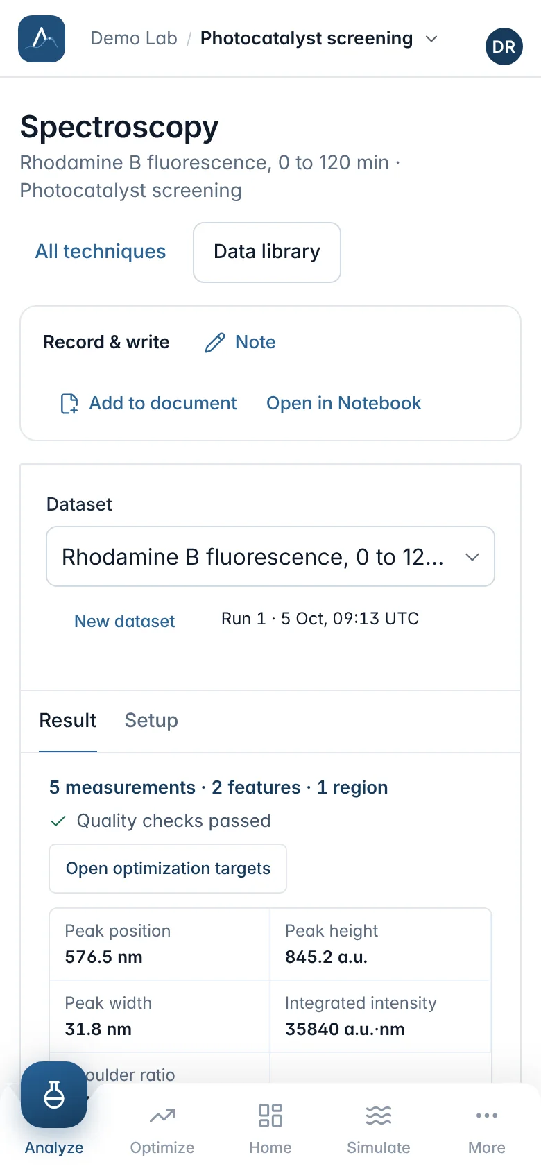
- The results table lists each value with its unit and uncertainty, and the quality checks the method ran. The columns used are named, so you can see what was read.
- The graph opens in Plot Studio, drawn in your saved style. Nothing there recomputes the result.
- Next on this data suggests the logical follow-up method with your settings carried over, for example “Name the peak types” or “qNMR purity” after NMR peaks.
- The Record & write bar adds a note, adds the result to a document or opens it in the Notebook.
When an analysis fails
A failed run says why. When the problem is in the setup, the message names a reason and what to fix; the file and the run stay in Data, and Fix setup and re-run opens the setup with your previous choices.
| Reason | What to do |
|---|---|
column_not_found | A selected column was not found in the file. Re-open the setup and pick the columns again from the preview. |
columns_same | The x axis and the signal are the same column. Choose two different columns. |
unit_missing | Enter a unit for both columns (a.u. for arbitrary units, 1 for dimensionless). |
unit_not_recognised | Use a standard symbol such as nm, s, mV or counts, a.u. for arbitrary units, or 1 for dimensionless. |
not_a_table | The file could not be read as a table of numbers with a header row. |
non_numeric_values | A selected column has empty or non-numeric values (text, blanks or NaN). Choose columns that contain only numbers, or clean those rows. |
too_few_points | The selected columns need at least two numeric rows. |
Other failures are reported in plain words: the analysis type does not support this input, the file is too large for this analysis, the analysis took too long and was stopped, or the analysis service is not ready (try again in a few minutes).
Not available yet
Some techniques are described in AcquiLAB's skill catalogue as specifications but cannot run yet, among them impedance spectra you measured (EIS; the Randles circuit exists as a simulation), GC-MS and LC-MS, DLS and zeta potential, DSC and TGA, ELISA, qPCR, flow cytometry, western blots, rheology and mechanical testing. AcquiLAB says so instead of guessing; they are planned.